What’s in a $&!#* vector?

TLDR:

• 2️⃣ We’re gonna check out two methods for explaining text embeddings and similarities or differences between texts
• 🧑‍🏫 Method 1 explains decisions by binding sub-embeddings to interpretable concepts, method 2 highlights tokens with integrated gradients

Some Keyphrases: Text embeddings, explainability, explainable similarity, representation learning

Intro

Goal of a $&!#*¹ vector

Capturing the meaning of a text as a vector (aka representation, or embedding, if you will) is an important goal of NLP research. With good vectors, we can perform important NLP tasks efficiently: search/information retrieval, clustering, evaluation, retrieval-augmented generation with LLMs (RAG), classification, and what not.

Why explain a $&!#* vector?

Obviously, in the age of BERT and LLMs, we do have methods that can well map text to a vector. While that’s pretty cool and also useful, at one point, we may have to explain why our model considers two texts are similar, or not. As an hypothetical edge case, think of a court where we’d have to argue why our model returned a “wrong” text that somehow led to some sort of legal mess further downstream.

So let’s dive into two cool methods for interpretation of embeddings.

The first method aims at understanding the text embedding vector space itself, and the second aims at understanding how tokens contribute to overall similarity. We’ll call those two:

1. Decision space explanation with multi feature embeddings and metric distillation. Code, Paper

2. Input space explanation to find salient phrase pairs. Code, Paper

Don’t worry, we’ll keep this post light-hearted, so that you won’t need to digest much math for understanding.

Decision explanation space with distillation

This is basically what I tinkered with in the last part of my PhD thesis. A motivation was to get some high-level explanation on similarity decisions and compose the overall similarity from aspectual sub-similarities.

Indeed, we’d like to search for explanations directly in the decision space, as us humans often also seek higher-level explanations to explain a decision: So we’d want to have something like “These documents are similar because they’re about the same topics”. “These documents are dissimilar because they’re contradicting each other”. And so on. This should happen in a faithful way, that is, the overall similarity of two texts should be derived from the aspectual similarities.

Let’s sketch the basic idea in this figure:

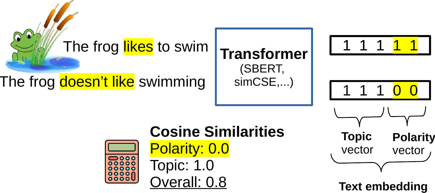
In the example, the overall similarity is 0.8, explained as follows: the sentences have the same topic (1.0), but opposing polarity (0.0). These sub-vectors (aka sub-embeddings, or features) compose the full text representation, so we can exactly trace how they’re weighted in the final score!

For customization you’d have to implement some simple and interpreable metrics that measure text similarity in different aspects. Then we can bind these metrics to sub-vectors and start learning to divide the text space into sub-spaces that capture different attributes that we’re interested in! In the end, we can trace the full similarity computation back to our high-level features.

A strength of this approach may also be a drawback: There’s lots of freedom in how you design your interpretable metrics, which can require some time for exploration to figure out what works and what not.

Input space explanation with integration

This is a cool work by Lukas Moeller et al. Here we’d like to know the input features that have the most impact on a decision. It’s sort of one of the most popular interpretability goals, where people want to highlight the input features that a model thinks are important. This is about how it’s done in this case:

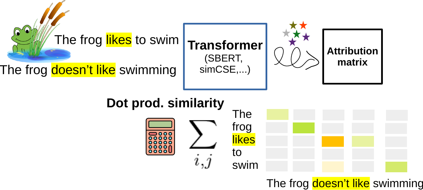
The sparkling stars stand for some magic (that is math) that’s happening in the process. It gives us a so-called attribution matrix. The matrix approximates the full similarity function of two texts, in a token-decomposed way! That means, we can check out how every pair of words contributes to the overall similarity.

What’s in the magic? The matrix is found with the method of “integrated gradients”: Starting from a neutral input, we kind of view how the gradients change when gradually going to our real input, integrating the path with respect to each input token. Since by integrating a gradient we sort of end up at our actual model function, we have all rights to call this approach faithful.

Like in every method, there’s may be also some downsides to this approach: we’d need i) to run some iterative approximations which makes the method not efficient and ii) we’d have to stick using dot-product as a similarity measure. This can lower the results on benchmarks by a tiny bit, and can reduce the practical usage in case we want to run the method for a lot of pairs.²

Other approaches:

There’s also interesting other papers about vectors and interpretability: Vivi Nastase shows that matrix structures can potentially capture some phenomena better than vectors. Jannis Vasmas and Rico Sennrich show that to detect meaningful differences between tokens of documents, it’s quite effective to simply use a greedy token matching similar to what’s done by BERTScore.

References

Click to extend

SBERT studies Meaning Representations: Decomposing Sentence Embeddings into Explainable Semantic Features (Opitz & Frank, AACL-IJCNLP 2022)

An Attribution Method for Siamese Encoders (Moeller et al., EMNLP 2023)

Footnotes

1. The “$&!#* vector” is derived from a quote ascribed to R. Mooney, see also this presentation. ↩

2. A later paper by the same authors seems to mitigate some of these issues. ↩